Hello, sp.fem!
This is the documentation of a simple finite element assembler library written in Python 2.7. The library is useful for quickly creating numerical solvers for various PDE-based models.
The library is currently work-in-progress and there is a fair amount of work to be done until it can be considered complete. The current state is however more than usable.
Getting started
You can download the library and get started by running the following commands
git clone https://github.com/kinnala/sp.fem
cd sp.fem
If you are a well-seasoned Python developer you may look into the contents of requirements.txt, check that you have all the required libraries and do whatever you wish.
Otherwise, we suggest that you use miniconda for managing Python virtual environments and installing packages. You can download and install miniconda by running
make install-conda
Next you can create a new conda environment spfemenv and install the required packages by running
make dev-install
The newly created virtual environment can be activated by writing
source activate spfemenv
Optionally, in order to use the geometry module, you should install MeshPy dependency by running
pip install meshpy
Tutorial
We begin by importing the necessary library functions.
from spfem.mesh import MeshTri
from spfem.assembly import AssemblerElement
from spfem.element import ElementTriP1
from spfem.utils import direct
Let us solve the Poisson equation in a unit square \(\Omega = [0,1]^2\) with unit loading. We can obtain a mesh of the unit square and refine it six times by
m = MeshTri()
m.refine(6)
By default, the initializer of spfem.mesh.MeshTri returns a mesh of the
unit square with two elements. The spfem.mesh.MeshTri.refine() method
refines the mesh by splitting each triangle into four subtriangles. Let us
denote the finite element mesh by \(\mathcal{T}_h\) and an arbitrary element
by \(K\).
The governing equation is
and it is combined with the boundary condition
The weak formulation reads: find \(u \in H^1_0(\Omega)\) satisfying
for every \(v \in H^1_0(\Omega)\).
We use a conforming piecewise linear finite element approximation space
The finite element method reads: find \(u_h \in V_h\) satisfying
for every \(v_h \in V_h\). A typical approach to impose the boundary condition \(u_h=0\) (which is implicitly included in the definition of \(V_h\)) is to initially build the matrix and the vector corresponding to the discrete space
and afterwards remove the rows and columns corresponding to the boundary nodes. An assembler object corresponding to the mesh \(\mathcal{T}_h\) and the discrete space \(W_h\) can be initialized by
a = AssemblerElement(m, ElementTriP1())
and the stiffness matrix and the load vector can be assembled by writing
A = a.iasm(lambda du, dv: du[0]*dv[0] + du[1]*dv[1])
b = a.iasm(lambda v: 1.0*v)
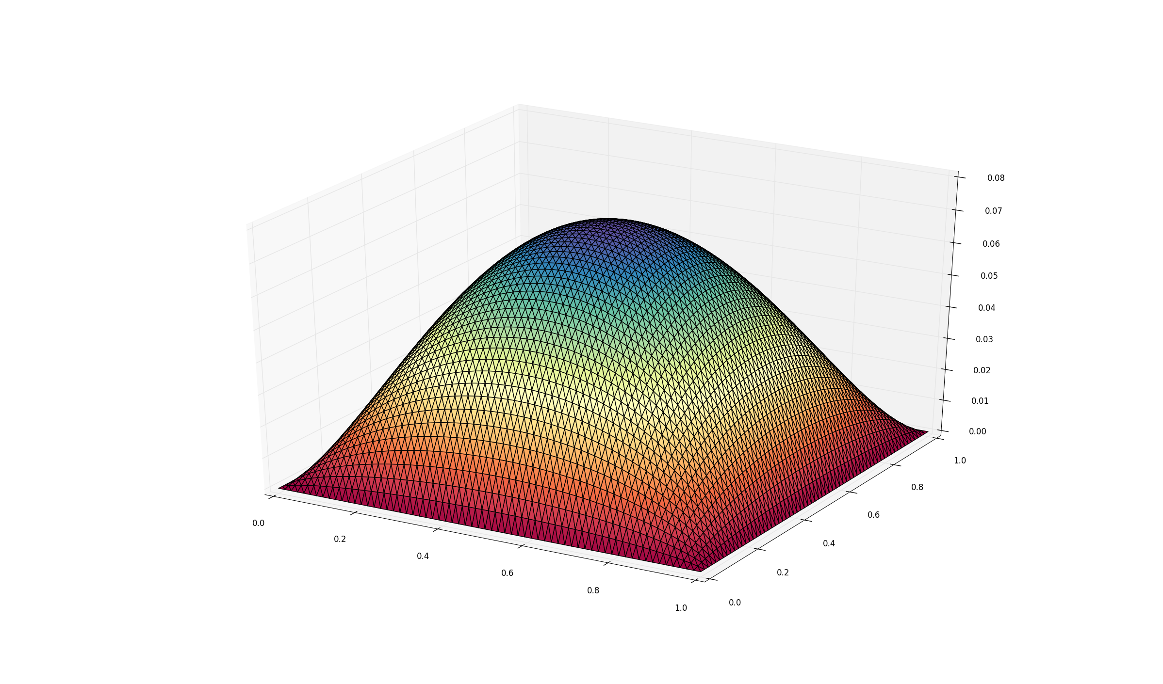
Finally you can solve the resulting linear system and visualize the resulting solution by
x = direct(A, b, I=m.interior_nodes())
m.plot3(x)
m.show()
Classes
This section contains documentation generated automatically from the source code of the relevant classes.
fem.mesh
Classes that represent different types of meshes.
Currently implemented mesh types are
spfem.mesh.MeshTri, a triangular meshspfem.mesh.MeshTet, a tetrahedral meshspfem.mesh.MeshQuad, a mesh consisting of quadrilateralsspfem.mesh.MeshLine, one-dimensional mesh
Examples
Obtain a three times refined mesh of the unit square and draw it.
from spfem.mesh import MeshTri
m = MeshTri()
m.refine(3)
m.draw()
m.show()
-
class
spfem.mesh.Mesh(p, t)¶ Abstract finite element mesh class.
-
dim()¶ Return the spatial dimension of the mesh.
-
remove_elements(ix)¶ Return new mesh with elements removed based on their indices.
Parameters: ix : numpy array
List of element indices to remove.
-
scale(scale)¶ Scale the mesh.
Parameters: scale : float OR tuple of size dim
Scale each dimension by a factor. If a floating point number is provided, same scale is used for each dimension.
-
show()¶ Call the correct pyplot/mayavi show commands after plotting.
-
translate(vec)¶ Translate the mesh.
Parameters: vec : tuple of size dim
Translate the mesh by a vector.
-
-
class
spfem.mesh.MeshLine(p=None, t=None, validate=True)¶ One-dimensional mesh.
-
plot(u, color='ko-')¶ Plot a function defined on the nodes of the mesh.
-
refine(N=1)¶ Perform one or more uniform refines on the mesh.
-
-
class
spfem.mesh.MeshQuad(p=None, t=None, validate=True)¶ A mesh consisting of quadrilateral elements.
-
boundary_facets()¶ Return an array of boundary facet indices.
-
boundary_nodes()¶ Return an array of boundary node indices.
-
draw()¶ Draw the mesh.
-
facets_satisfying(test)¶ Return facets whose midpoints satisfy some condition.
-
interior_nodes()¶ Return an array of interior node indices.
-
jiggle(z=None)¶ Jiggle the interior nodes of the mesh.
-
nodes_satisfying(test)¶ Return nodes that satisfy some condition.
-
param()¶ Return mesh parameter.
-
plot(z, smooth=False)¶ Visualize nodal or elemental function (2d).
-
plot3(z, smooth=False)¶ Visualize nodal function (3d i.e. three axes).
-
refine(N=1)¶ Perform one or more refines on the mesh.
-
splitquads(z)¶ Split each quad into a triangle and return MeshTri.
-
-
class
spfem.mesh.MeshTet(p=None, t=None, validate=True)¶ Tetrahedral mesh.
-
boundary_edges()¶ Return an array of boundary edge indices.
-
boundary_facets()¶ Return an array of boundary facet indices.
-
boundary_nodes()¶ Return an array of boundary node indices.
-
build_mappings()¶ Build element-to-facet, element-to-edges, etc. mappings.
-
draw(test=None, u=None)¶ Draw all tetrahedra.
-
draw_edges()¶ Draw all edges in a wireframe representation.
-
draw_facets(test=None, u=None)¶ Draw all facets.
-
draw_vertices()¶ Draw all vertices using mplot3d.
-
edges_satisfying(test)¶ Return edges whose midpoints satisfy some condition.
-
facets_satisfying(test)¶ Return facets whose midpoints satisfy some condition.
-
interior_nodes()¶ Return an array of interior node indices.
-
nodes_satisfying(test)¶ Return nodes that satisfy some condition.
-
param()¶ Return (maximum) mesh parameter.
-
refine(N=1)¶ Perform one or more refines on the mesh.
-
shapereg()¶ Return the largest shape-regularity constant.
-
-
class
spfem.mesh.MeshTri(p=None, t=None, validate=True)¶ Triangular mesh.
-
boundary_facets()¶ Return an array of boundary facet indices.
-
boundary_nodes()¶ Return an array of boundary node indices.
-
draw(nofig=False)¶ Draw the mesh.
-
draw_nodes(nodes, mark='bo')¶ Highlight some nodes.
-
elements_satisfying(test)¶ Return elements whose midpoints satisfy some condition.
-
facets_satisfying(test)¶ Return facets whose midpoints satisfy some condition.
-
interior_facets()¶ Return an array of interior facet indices.
-
interior_nodes()¶ Return an array of interior node indices.
-
interpolator(x)¶ Return a function which interpolates values with P1 basis.
-
nodes_satisfying(test)¶ Return nodes that satisfy some condition.
-
param()¶ Return mesh parameter.
-
plot(z, smooth=False, nofig=False, zlim=None)¶ Visualize nodal or elemental function (2d).
-
plot3(z, smooth=False)¶ Visualize nodal function (3d i.e. three axes).
-
refine(N=1)¶ Perform one or more refines on the mesh.
-
fem.asm
Assembly of matrices related to linear and bilinear forms.
Examples
Assemble the stiffness matrix related to the Poisson problem using the piecewise linear elements.
from spfem.mesh import MeshTri
from spfem.assembly import AssemblerElement
from spfem.element import ElementTriP1

m = MeshTri()
m.refine(3)
e = ElementTriP1()
a = AssemblerElement(m, e)

def bilinear_form(du, dv):
    return du[0]*dv[0] + du[1]*dv[1]

K = a.iasm(bilinear_form)
fem.element
The finite element definitions.
- Try for example the following actual implementations:
-
class
spfem.element.AbstractElement¶ This will replace ElementGlobal in the future.
-
dim= 0¶ Spatial dimension
-
e_dofs= 0¶ Number of edge dofs (3d only)
-
f_dofs= 0¶ Number of facet dofs (2d and 3d only)
-
i_dofs= 0¶ Number of interior dofs
-
maxdeg= 0¶ Maximum polynomial degree
-
n_dofs= 0¶ Number of nodal dofs
-
-
class
spfem.element.AbstractElementArgyris¶ Argyris element for fourth-order problems.
-
class
spfem.element.AbstractElementMorley¶ Morley element for fourth-order problems.
-
class
spfem.element.AbstractElementTriPp(p=1)¶ Triangular Pp element, Lagrange DOFs.
-
class
spfem.element.Element¶ Abstract finite element class.
-
dim= 0¶ Spatial dimension
-
e_dofs= 0¶ Number of edge dofs (3d only)
-
f_dofs= 0¶ Number of facet dofs (2d and 3d only)
-
gbasis(X, i, tind)¶ Returns global basis functions evaluated at some local points.
-
i_dofs= 0¶ Number of interior dofs
-
lbasis(X, i)¶ Returns local basis functions evaluated at some local points.
-
maxdeg= 0¶ Maximum polynomial degree
-
n_dofs= 0¶ Number of nodal dofs
-
-
class
spfem.element.ElementGlobal¶ An element defined globally. These elements are used by
spfem.assembly.AssemblerGlobal.-
gbasis(mesh, qps, k)¶ Return the global basis functions of an element evaluated at the given quadrature points.
Parameters: mesh
The
spfem.mesh.Meshobject.qps : dict of global quadrature points
The global quadrature points in the element k.
k : int
The index of the element in mesh structure.
Returns: u : dict
A dictionary with integer keys from 0 to Nbfun. Here u[i] contains the values of the i’th basis function of the element k evaluated at the given quadrature points (np.array).
du : dict
The first derivatives. The actual contents are 100% defined by the element implementation although du[i] should correspond to the i’th basis function.
ddu : dict
The second derivatives. The actual contents are 100% defined by the element implementation although ddu[i] should correspond to the i’th basis function.
-
visualize_basis_2d(show_du=False, show_ddu=False, save_figures=False)¶ Draw the basis functions given by self.gbasis. Only for 2D triangular elements. For debugging purposes.
-
-
class
spfem.element.ElementGlobalArgyris(optimize_u=False, optimize_du=False, optimize_ddu=False)¶ Argyris element for fourth-order problems.
-
class
spfem.element.ElementGlobalDGTriP0¶ A triangular constant DG element.
-
class
spfem.element.ElementGlobalDGTriP1¶ A triangular first-order DG element.
-
class
spfem.element.ElementGlobalDGTriP2¶ A triangular second-order DG element.
-
class
spfem.element.ElementGlobalDGTriP3¶ A triangular third-order DG element.
-
class
spfem.element.ElementGlobalMorley¶ Morley element for fourth-order problems.
-
class
spfem.element.ElementGlobalTriP1¶ The simplest possible globally defined elements. This should only be used for debugging purposes. Use
ElementTriP1instead.
-
class
spfem.element.ElementGlobalTriP2¶ Second-order triangular elements, globally defined version. This should only be used for debugging purposes. Use
ElementTriP2instead.
-
class
spfem.element.ElementH1¶ Abstract \(H^1\) conforming finite element.
-
class
spfem.element.ElementH1Vec(elem)¶ Convert \(H^1\) element to vectorial \(H^1\) element.
-
class
spfem.element.ElementHdiv¶ Abstract \(H_{div}\) conforming finite element.
-
class
spfem.element.ElementLineP1¶ Linear element for one dimension.
-
class
spfem.element.ElementQ1¶ Simplest quadrilateral element.
-
class
spfem.element.ElementQ2¶ Second order quadrilateral element.
-
class
spfem.element.ElementTetDG(elem)¶ Convert a H1 tetrahedral element into a DG element. All DOFs are converted to interior DOFs.
-
class
spfem.element.ElementTetP0¶ Piecewise constant element for tetrahedral mesh.
-
class
spfem.element.ElementTetP1¶ The simplest tetrahedral element.
-
class
spfem.element.ElementTetP2¶ The quadratic tetrahedral element.
-
class
spfem.element.ElementTriDG(elem)¶ Transform a H1 conforming triangular element into a discontinuous one by turning all DOFs into interior DOFs.
-
class
spfem.element.ElementTriMini¶ The MINI-element for triangular mesh.
-
class
spfem.element.ElementTriP0¶ Piecewise constant element for triangular mesh.
-
class
spfem.element.ElementTriP1¶ The simplest triangular element.
-
class
spfem.element.ElementTriP2¶ The quadratic triangular element.
-
class
spfem.element.ElementTriPp(p)¶ A somewhat slow implementation of hierarchical p-basis for triangular mesh.
-
class
spfem.element.ElementTriRT0¶ Lowest order Raviart-Thomas element for triangle.
fem.mapping
The mappings defining relationships between reference and global elements.
Currently these classes have quite a lot of undocumented behavior and untested code. The following mappings are implemented to some extent:
spfem.mapping.MappingAffine, the standard affine local-to-global mapping that can be used with triangular and tetrahedral elements.spfem.mapping.MappingQ1, the local-to-global mapping defined by the Q1 basis functions. This is required for quadrilateral meshes.
-
class
spfem.mapping.Mapping(mesh)¶ Abstract class for mappings.
-
F(X, tind)¶ Element local to global.
-
G(X, find)¶ Boundary local to global.
-
fem.utils
Utility functions.
-
class
spfem.utils.ConvergenceStudy(fname)¶ A module to simplify creating convergence studies. Uses *.pkl (pickle) files as key-value-type storage and enables simple plotting and fitting of linear functions on logarithmic scale.
-
spfem.utils.cell_shape(x, *rest)¶ Find out the shape of a cell array.
-
spfem.utils.cg(A, b, tol, maxiter, x0=None, I=None, pc='diag', verbose=True, viewiters=False)¶ Conjugate gradient solver wrapped for FEM purposes.
-
spfem.utils.const_cell(nparr, *arg)¶ Initialize a cell array (i.e. python dictionary) with the given parameter array/float by performing a deep copy.
Example. Initializing a cell array with zeroes.
>>> from fem.utils import const_cell
>>> const_cell(0.0, 3, 2)
{0: {0: 0.0, 1: 0.0}, 1: {0: 0.0, 1: 0.0}, 2: {0: 0.0, 1: 0.0}}
-
spfem.utils.direct(A, b, x=None, I=None, use_umfpack=True)¶ Solve system Ax=b with Dirichlet boundary conditions.
-
spfem.utils.gradient(u, mesh)¶ Compute the gradient of a piecewise linear function.
Tips
- Errors related to qt4, wx, mayavi, etc. can be sometimes fixed by simply changing environment variables or running ipython with the following flags:
ipython --gui=wx --pylab=wx
ETS_TOOLKIT=qt4 ipython --gui=wx --pylab=wx
- Simplest way to run tests is to discover them all using unittest as follows:
ipython -m unittest discover ./spfem
- In order to estimate test coverage you can install coverage.py and run it
pip install coverage
coverage run -m unittest discover ./spfem
coverage html
License
sp.fem is free software: you can redistribute it and/or modify it under the terms of the GNU Affero General Public License as published by the Free Software Foundation, either version 3 of the License, or (at your option) any later version.
sp.fem is distributed in the hope that it will be useful, but WITHOUT ANY WARRANTY; without even the implied warranty of MERCHANTABILITY or FITNESS FOR A PARTICULAR PURPOSE. See the GNU Affero General Public License for more details.
You should have received a copy of the GNU Affero General Public License along with sp.fem. If not, see <http://www.gnu.org/licenses/>.